1. Steps

1.1. Data preparation

1. Prepare the time slice $\textbf{X}_k(I\times J)$
2. Normalization: mean-centered, unit-variance

1.2. Time-slice based PCA modeling

1. Perform PCA on the time slice data
2. Choose the PC number according to the explained variance ratio
3. Calculate the SPE and its limit, $Ctr_k$

1.3. Time-segment based PCA modeling

1. Add the next time slice to the existing ones.
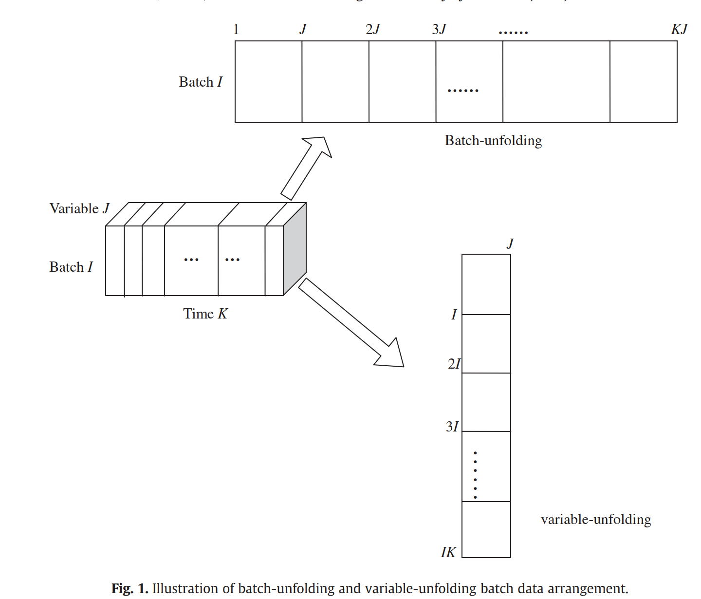
2. Variable-wise unfold the data within the current time region, $X_{v,k}(Ik × J)$
   
3. Calculate the confidence limit, $Ctr_{v,k}$

1.4. Compare model accuracy

1. Find the time $k^*$ from which 3 consecutive samples show $Ctr_{v, k}>\alpha Ctr_k$ ($\alpha$ is the relaxing factor)
2. The time slices before $k^*$ are denoted as one sub-phase
3. Remove the previous subspace, repeat Step 3 and 4 until all samples are assigned to a sub-phase.

2. Hotelling's $T^2$

Hotelling' $T^2$ can be used by simply replacing the SPE index. However, it may not reflect the time-varying underlying process characteristics as sensitively as SPE. Also, from the illustration results, the division may not significantly influence the T2 monitoring performance.

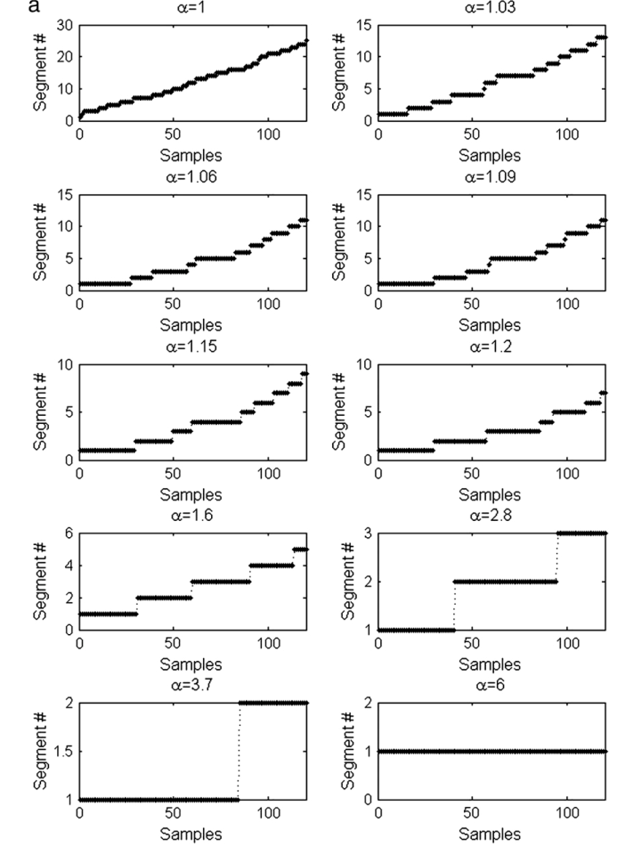
3. Relaxing factor $\alpha$

The relaxing factor $\alpha$ determines the loss tolerance of reconstruction power of time-segment model in comparison with the associated time-slice models. Larger $\alpha$ value means more reduction of reconstruction power is allowed, resulting in less number of monitoring models.

The relaxing factor reflects the compromise between model accuracy and model complexity. In general, the value of $\alpha$ can be set by trial and error so that each representative model will not cover too much process patterns to ensure the sensitiveness to the changes of process characteristics. However, up to now, there is no definite criterion or uniform standard to strictly quantify it.